Deep dive into the past performance of my portfolio
· 1711 words · 9 minutes read
When I set up my portfolio about a year ago, I based its composition on the recommendations laid out in Richard Ferri’s excellent book All About Asset Allocation. Once I knew what percentages I wanted to assign to bonds, equities from developed markets, emerging markets, etc… it was a matter of finding the matching funds on justETF.
However, I never bothered to actually test the past performance of the portfolio before investing my money. Although unlikely, maybe Richard Ferri is just saying a bunch of bollocks and his recommendations aren’t actually any good? Therefore, I decided to find out for myself just how well it had actually been performing in the past.
Read on to find out the answer.
Composition
For reasons I described in an earlier post titled An intro to passive investing, my portfolio is composed of solely index funds.
| ETF | Allocation | Index |
|---|---|---|
| iShares Core MSCI World | 49% | MSCI World |
| iShares MSCI World Small Cap | 14% | MSCI World Small Cap |
| Xtrackers MSCI Emerging Markets | 10% | MSCI Emerging Markets |
| Amundi ETF FTSE EPRA NAREIT Global | 9% | FTSE EPRA/NAREIT |
| Xtrackers Global Sovereign | 18% | FTSE World Government Bond Index |
The three MSCI indexes track the stock market, FTSE World Government Bond Index is a bond index and FTSE EPRA/NAREIT is an index for the real estate market.
Getting the historical data
The initial step in calculating the past performance of the portfolio is to get the historical values of its composing funds. As a first approach, we can go to Yahoo Finance and fetch the historical data for iShares Core MSCI World. However, the issue is that the funds are usually much younger than the indexes that they track. According to the factsheet, this particular fund was created in 2009. However, the MSCI World index was established in 1986!
Most indexes in the portfolio are actually pretty old:
- MSCI World: 1986
- MSCI World Small Cap: 2001
- MSCI Emerging Markets: 2001
- FTSE EPRA/NAREIT: 2005
- FTSE World Government Bond Index: 1986
To substantiate the validity of our simulation, we want to go back in time as far as possible. So our assignment becomes finding the historical values for the indexes in the portfolio as opposed to the funds themselves.
The MSCI indexes
Three of the funds in our portfolio track an MSCI index. It wasn’t too hard to find the historical data for these indexes as the company website has a page dedicated to historical data. You do have to launch an outdated Flash application, but this will allow you to download an Excel spreadsheet with the wanted data.
An interesting observation is that the historical data goes back further than the inception date of the index. For instance, the data for MSCI World starts in 1970 whereas the index was only created in 1986. To do this, they apply back-testing, meaning that they calculate how the index might have performed had it existed.
FTSE EPRA/NAREIT
The data for the FTSE EPRA/NAREIT index, the real estate part of the portfolio, was a bit harder to find. After a long search, I found a 66MB Zip file on the EPRA website that contains the data for all their indexes, from which I could extract the information I needed.
The data for this index starts in 1990. Therefore it’s not as old as some of the MSCI indexes but this is still far enough in time for our purposes.
FTSE World Government Bond Index
Finding the data for the FTSE World Government bond index was the most frustrating. It is seemingly only available through The Yield Book but it’s blocked by a paywall. Selling the historical data of their indexes must be an important aspect of their business model.
Instead, I opted to find the historical data for a fund that tracks the index but unfortunately I was unable to find a fund that was old enough.
As a last resort, I decided to use another bond index as a proxy for WGBI. After all, it’s important that a bond index is included in the analysis due to its stabilizing effect on the entire portfolio. I settled on the JP Morgan Government Bond Index, mainly because it was the most comparable bond index that I could find that had sufficient historical data available for free.
Like WGBI, it tracks investment-grade government bonds. A key difference though is that WGBI is global whereas our proxy, the JP Morgan Government Bond index, is only composed of US bonds.
To quantify the resemblance of the two indexes, I calculated that their correlation between 2013 and 2018 is 0.90. A higher correlation is preferred because it indicates that the two indexes are more alike. 0.90 is not ideal but it’s not terrible either. It will have to do as it’s the only other government bond index that I could find with sufficient data.
Preparing the data
Now that we have gathered the raw data, we need to prepare it for analysis. First, we must find the common time period between all the datasets. It turns out that we have all the data necessary to perform the simulation from February 1993 to December 2015. That’s almost 23 years in total, which gives us sufficient validation for how our portfolio behaves, both in times when the markets are peaking and when they’re crashing (e.g. in 2008).
Secondly, we need to convert all five datasets into the same format. I chose to convert them to CSV files as it’s a text format that can easily be processed by a program written in any programming language.
The simulation
We are now ready to start the simulation: if we had invested €1,000 in February 1993, how much would we have had in December 2015?
The answer is €3,375 or a 5.47% average annual return rate (AARR).
Instead of running the simulation in a spreadsheet, I created a small website called Backtest that runs the simulation for me. As a professional web developer, I found this method to be easier, and it provided a means to share the information with others in a more aesthetic way (although I recognize there is room for improvement when it comes to its visual design).
Comparing simulations with and without rebalancing
As I explain in A crash course on asset allocation, rebalancing is a mechanism where you periodically restore the allocation in your portfolio. Indeed, because the price of each fund in your portfolio changes differently, over time the weightings of the funds will diverge from the allocation that you initially defined. For instance, if the real estate market has been doing really well and grew 30% in 6 months, the real estate portion of the portfolio might now represent 15% of the total value instead of the 10% that you initially defined. To rebalance, you would sell some shares of the real estate fund and buy some shares of the other funds to bring its allocation back to 10%. Theory says that rebalancing will result in a higher total return because it forces us to sell high and buy low.
Therefore, I did a second run where the portfolio is rebalanced every year. As expected, this improved the performance and we ended up with €3,881 or an AARR of 6.12%.
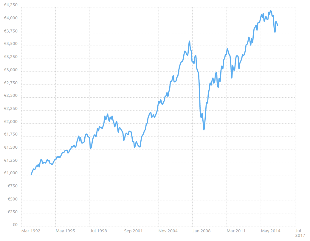
Evolution of the total value of the portfolio when rebalancing yearly.
Limitations of the analysis
We made several simplifications in our model that have an impact on the accuracy of the outcome:
- Due to a lack of available data, I had to use a proxy index for the FTSE World Government Bond Index. We calculated that for the last 5 years, the correlation between the two indexes was 0.90. This makes them fairly similar, but having the actual index data would increase the accuracy of the simulations.
- I did not include dividend payments. Each of the funds in the portfolio pays out dividends, that are then reinvested. Including these gains in the analysis would positively impact the return.
- I did not include losses due to taxes and trading fees. These are highly dependent on time (tax laws change all the time) and the residing country of the investor. Therefore, it would make this analysis much more complicated and too tailored to my specific case. However, we do know that they would negatively impact the return.
- The model assumes that it is possible to buy fractional parts of an index. In reality, ETFs are traded like shares and only purchasable as whole units, i.e. you can’t buy 0.4 of an ETF. However, this effect becomes negligible when investing sufficiently large amounts so it doesn’t really affect the validity of the result.
Conclusion
| Rebalancing strategy | Average annual return rate (AARR) |
|---|---|
| No rebalancing | 5.47% |
| Yearly rebalancing | 6.12% |
Past performance cannot guarantee future outcomes but it can give a good indication. The most important result of our simulation is that our portfolio has given an average return of around 6% during a period of 23 years. It’s fair to assume that the performance for the following years will be similar.
Topics for future articles
Following this research, there are a couple of topics that I want to explore further in a future post:
- impact of dividends on total return. We did not include dividend payouts in this simulation. However, I expect that reinvested dividends will have a non-negligible positive effect on the total return. Calculating the impact is a topic for a future post.
- impact of rebalancing strategies. We already saw here that rebalancing has a big impact on the total return of a portfolio. Are some strategies better than others? Is it better to rebalance monthly, quarterly, yearly or even two-yearly?
- optimal asset allocation for the portfolio. What would be the optimal allocation if we want to maximize returns? What if we instead wish to maximize the Sharpe ratio or Calmar ratio? What would be the effect of reducing or increasing the allocation of bonds in the portfolio?
My questions to you
Finally, I have two requests for you. I am still on the lookout for the data that I couldn’t find. Please let me know if you have access to:
- the historical data for the FTSE World Government Bond Index,
- the historical data for the FTSE EPRA/NAREIT index for 2016 and onwards,